Back-propagation learning for multi-layer feedforward neural network

Below are the objectives of this post:

1. What is multi-layer feed-forward neural network
2. Discuss back-propagation algorithm which is used to train it
3. Implement what we discuss in python to gain better understanding
4. Execute the implementation for a binary classification use-case to get a practical perspective

Multi-layer feed-forward neural network consists of multiple layers of artificial neurons.  As the name suggests, one layer acts as input to the layer after it and hence feed-forward. But at the same time the learning of weights of each unit in hidden layer happens backwards and hence back-propagation learning.

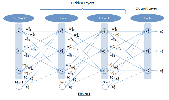
For this discussion let us consider the neural network shown in Figure 1. It has three neural units in each layers and b1, b2, b3 are included as units (with input as 1) for bias. Figure 1 has one input layer, one output layer (layer L) and 2 hidden layers (L-1 and L-2).

Below are two high level steps in building a multi-layer feed-forward neural network model. These steps are executed iteratively:

1. Feed-forward: Data from input layer is fed forward through each layer and then output is generated in the final layer.
2. Back-propagation: This is the learning step. Once the output is generated, the error is calculated w.r.t. the expected output and then this error is propagated in backwards direction to adjust the weights to reduce the error. This is the learning step.

Let us discuss each of the steps in detail:

1. Feed-forward: On a high-level two steps are executed at every unit during feed-forward:
   1. Weighted sum of all inputs is calculated (including bias). Figure 2 shows a detailed view of  unit. is the input to  and is weighted sum of all three activations (non-linearized output) and the bias from the previous layer i.e. 
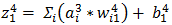
   2. Then non-linearization of the input (calculated in #1 above) is done i.e. . Here  is the output of the unit as shown in Figure 2. 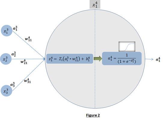Similarly, each unit receives the inputs from previous layers and passes the non-linearized output to the next layer. The functions for non-linearization are chosen such that they are differentiable (we will answer ‘why?’ while talking about back-propagation). Below are few notations to keep in mind for generalization:
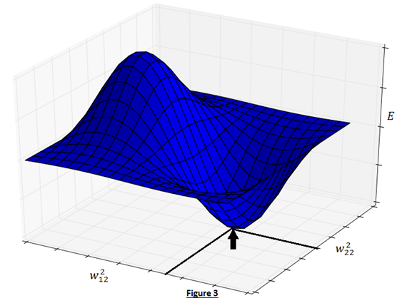
2. Back-propagation learning: The overall objective of backpropagation learning is to learn combination of weights which minimizes the output error. The error between actual output and the desired output is reduced (in each iteration) by doing supervised adjustment in weights.  We will not be able to visualize the space with all weights and error but for intuitive understanding let’s see error with two weights in Figure 3. Objective is to learn weights such that value of E is minimum (as pointed by arrow in Figure 3).Now the question is, how to learn this combination of weights? We will do this learning using gradient descent so that weights learnt, in each iteration, move ‘generated output’ in the direction towards the ‘expected output’. As gradient descent requires the cost function to be differentiable, we have taken sigmoid as activation function.Now let us write the above understanding in maths so that we can implement it later in python. For neural network in Figure 1, the error function is defined as:  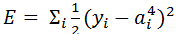where  is the expected output of i^th unit of output layer. 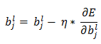We need to find   for all units of all layers and adjust each weight as below:

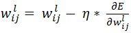
where  is the learning rate.

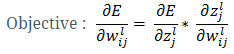
Let us derive an expression for  which can be generalized to any weight and any layer in the network.

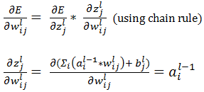
Let us call  as  , which represents change in error with unit change in input to j^th unit of l^th layer. So,

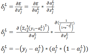
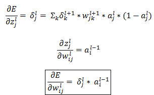
Let us compute  if l = ‘L’ i.e. the output layer for any neural network (L= 4 in Figure 1) then,

Now let’s derive an expression for  for hidden layers:

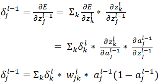
Based on the above equation we can calculate  for all units of all layers, provided the same has been calculated for the layer ahead. So we will have to calculate it backwards. So let’s conclude:

Similarly, we will derive expression for    as:

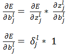
Finally, the weight updates happens as earlier discussed:

For online learning, one example is introduced at a time and weights are updated incrementally (for each example).

For batch learning, a batch of examples is introduced and weights are updated only once for the whole batch. So an average of gradients for all examples is used to update the weights.

Below is the python implementation for feed-forward backpropagation in batch learning mode:

"""
Author: Ashish Verma
This code was developed to give a clear understanding of what goes behind the curtains in multi-layer feedforward backpropagation neural network.
Feel free to use/modify/improve/etc.

Caution: This may not be an efficient code for production related usage so thoroughly review and test the code before any usage.
"""

import numpy as np
import matplotlib.pyplot as plt
from sklearn import preprocessing
from scipy import spatial

class multiLayerFeedForwardNN:
    def __init__(self, listOfNeuronsEachLayer):
        self.listOfNeuronsEachLayer = listOfNeuronsEachLayer
        self.dictOfWeightsEachLayer = {}
        self.dictOfActivationsEachLayer = {}
        self.dictOfDeltaEachLayer = {}
        self.dictOfZeeEachLayer = {}
        self.dictOfGradientsEachLayer = {}
        self.listAvgCost = []
        #Initialize weights with random values (this also includes bias terms)
        for iLayer in range(1,len(listOfNeuronsEachLayer)):
            self.dictOfWeightsEachLayer[iLayer + 1] = np.mat(np.random.random((listOfNeuronsEachLayer[iLayer], listOfNeuronsEachLayer[iLayer-1]+1)))

    def sigmoidFunc(self, z):
        result = 1/(1 + np.exp(-1*z))
        return result

    def feedForward(self, inputChunk):
        #Loop over all layers
        for iLayer in range(1, len(self.listOfNeuronsEachLayer)):
            #Save input itself as the activation for the input layer. We will use it later in the code
            if(iLayer == 1):
                self.dictOfActivationsEachLayer[1] = inputChunk
            #Insert extra element for bias having value 1 in input elements
            inputChunk = np.hstack([inputChunk, np.mat(np.ones(len(inputChunk))).T])
            #Calculate z using matrix multiplication of weights and inputs
            self.dictOfZeeEachLayer[iLayer+1] = np.dot(inputChunk, self.dictOfWeightsEachLayer[iLayer+1].T)
            #Calculate 'a' after non-linearizing z
            self.dictOfActivationsEachLayer[iLayer+1] = self.sigmoidFunc(self.dictOfZeeEachLayer[iLayer+1])
            #Consider activation of the current layer as input to the next layer
            inputChunk = self.dictOfActivationsEachLayer[iLayer+1]

    def calculateDelta(self, outputChunk):
        #Calculate delta backwards (output layer to 2nd layer)
        for iLayer in range(len(self.listOfNeuronsEachLayer),1,-1):
            #For last layer calculate delta
            if(iLayer == len(self.listOfNeuronsEachLayer)):
                self.dictOfDeltaEachLayer[iLayer] = np.multiply((self.dictOfActivationsEachLayer[iLayer] - outputChunk), np.multiply(self.dictOfActivationsEachLayer[iLayer],(1-self.dictOfActivationsEachLayer[iLayer])))
            #For rest of the layers calculate delta using delta of next layer
            else:
                wDelta = np.dot(self.dictOfDeltaEachLayer[iLayer+1], np.delete(self.dictOfWeightsEachLayer[iLayer + 1],self.dictOfWeightsEachLayer[iLayer + 1].shape[1]-1,1))
                dadz = np.multiply(self.dictOfActivationsEachLayer[iLayer],(1-self.dictOfActivationsEachLayer[iLayer]))
                self.dictOfDeltaEachLayer[iLayer] = np.multiply(wDelta, dadz)

    def calculateErrorGradient(self):
        #Calculate error gradient for all layers
        for iLayer in range(2,len(self.listOfNeuronsEachLayer)+1):
            #Gradient w.r.t all weights
            self.dictOfGradientsEachLayer[iLayer] = np.dot(self.dictOfDeltaEachLayer[iLayer].T,self.dictOfActivationsEachLayer[iLayer-1])
            #Gradient w.r.t. biases and add it to the other gradients
            self.dictOfGradientsEachLayer[iLayer] = np.hstack([self.dictOfGradientsEachLayer[iLayer], np.sum(self.dictOfDeltaEachLayer[iLayer],0).T])

    def updateWeights(self, learningRate):
        #For all layers update weights using average of gradients over all examples
        for iLayer in range(2, len(self.listOfNeuronsEachLayer)+1):
            self.dictOfWeightsEachLayer[iLayer] = self.dictOfWeightsEachLayer[iLayer] - (learningRate/len(self.dictOfActivationsEachLayer[1]))*self.dictOfGradientsEachLayer[iLayer]

    def calculateAverageCost(self, actualOutput, expectedOutput):
        #Calculate average of error function
        avgOverLayer = np.average([(1/2.)*x**2 for x in np.array(actualOutput-expectedOutput)],1)
        return np.average(avgOverLayer)            

    def trainBatchFFBP(self, learningRate, inputData, outputData, miniBatchSize, maxIterations):
        #If the size of the data is large and resources are less, then divide it into batches for computation.
        #Define batch size accordingly or leave empty if data size is not big
        if(miniBatchSize == ''):
            miniBatchSize = len(inputData)
        #Initialize iteration counter
        iterations = 0
        #Iterate over all examples 'maxIterations' number of times
        #We can even let the program iterate untill the desired error reduction is achieved (this code doesn't implement it).
        for iterations in range(maxIterations):
            #iBatch takes care of dividing the full data in batches (if we chose to, incase the data is big)
            startRecord = 0
            for iBatch in range((len(inputData)/miniBatchSize)):
                endRecord = startRecord + miniBatchSize
                inputChunk = inputData[startRecord:endRecord]
                outputChunk = outputData[startRecord:endRecord]
                self.feedForward(inputChunk)
                self.calculateDelta(outputChunk)
                self.calculateErrorGradient()
                self.updateWeights(learningRate)
                startRecord = endRecord
                #print "iBatch", iBatch
                #--------------Just stack up all calculated output for average error calculation-----------------#
                if(iBatch == 0):
                    activationMat = self.dictOfActivationsEachLayer[len(self.listOfNeuronsEachLayer)].copy()
                else:
                    activationMat = np.vstack([activationMat,self.dictOfActivationsEachLayer[self.listOfNeuronsEachLayer]])
                #------------------------------------------------------------------------------------------------#
            if(endRecord < len(inputData)):
                inputChunk = inputData[startRecord:]
                outputChunk = outputData[startRecord:]
                self.feedForward(inputChunk)
                self.calculateDelta(outputChunk)
                self.calculateErrorGradient()
                self.updateWeights(learningRate)
                activationMat = np.vstack([activationMat,self.dictOfActivationsEachLayer[self.listOfNeuronsEachLayer]])
            self.listAvgCost.append(self.calculateAverageCost(activationMat, outputData))
            iterations = iterations + 1
            print iterations

Now, let us use the implementation for a binary classification task. We will be using the dataset obtained from https://archive.ics.uci.edu/ml/datasets/Ionosphere.

Ionosphere dataset’s output is either ‘g’ (good) or ‘b’ (bad). Let’s replace ‘g’ by 1 and ‘b’ by 0. This dataset has 34 features as input, so the input layer will have 34 neurons and we are using sigmoid activation function so we will be taking 1 neuron in output layer for binary classification.

#Import dataset
dataset = np.genfromtxt ('C:\Research\BlogPloration\BackPropogation\ComparisonDataset\ionosphere.csv', delimiter=",")

#Initialize 'multiLayerFeedForwardNN' with 34, 27 and 1 neurons in input, hidden and output layers respectively
objMLFFNN = multiLayerFeedForwardNN([34,27,1])
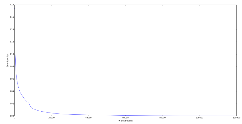
#Start training with learning rate as 0.5 and 120,000 iterations
objMLFFNN.trainBatchFFBP(0.5, np.mat(dataset[:,:34]), np.mat(dataset[:,34]).T,'', 120000)

This NN model fits the data fully. Let’s look at the plot of ‘error function value’ calculated with iterations during training. Error for every iteration is stored in ‘listAvgCost’.

Note: In order to keep things simple, I haven’t talked about regularization term and other aspects. I would suggest the readers to study further once the basic is ‘very’ clear.

Logistic Regression – Part 2

This is the 2^nd part of a two part series about Logistic Regression. In the last post – Logistic Regression – Part 1, we talked about what is logistic regression and why we need it. In this post we will talk about how to implement it in python. We will also execute it over a letter recognition dataset.

As it was mentioned in the last post, we will use Newton’s Method for estimating parameters of logistic regression. From the current available methods it is not possible to find the maxima by just equating derivative of the likelihood function to zero so we will use Newton’s method to converge to estimates iteratively.

Some equations that we will implement in our code:

Below is what the iteration in Newton’s method becomes:

where, first derivative w.r.t. one of the parameters is:

So, generalized representation for first derivative is:

Second derivative is:

So, generalized representation for second derivative becomes:

Take first and second derivatives of log likelihood function w.r.t. the parameter(s) to be estimated. Fit them in the above equation related to Newton’s method and find the next estimated values for parameter(s). This goes on iteratively till the values of estimates stop changing over iterations.

Now let’s look at the implementation in python. This is an implementation to understand logistic regression in a better way and by no means was this aimed at writing an efficient code. I have tried to comment the code well enough to give a good idea of what’s happening.

# -*- coding: utf-8 -*-

"""
Author: Ashish Verma
This code does logistic regression using newton's method for binary response variable
This code was developed to give a clear understanding of what goes behind the curtains in logistic regression using newton's method.
Feel free to use/modify/improve/etc. but beware that this may not be efficient for production related usage (especially where data is large).

This code is developed only for a binary response variable. If the classes are other than 0 and 1, then you'll have to transform them.
"""

import pandas as pd
import numpy as np
from numpy.linalg import inv
from sklearn import metrics

class logisticRegression:
    def __init__(self,X):
        #Estimated parameters are stored in 'newEstimatedParameters'. An extra element has been increased to store the intercept
        self.newEstimatedParameters = np.zeros(X.shape[1]+1)
        self.oldEstimatedParameters = []
        #self.probability is where final probability of the data is stored after convergence
        self.probability = []

    #This function contains one iteration update for parameters using newton's method.
    def newtonMethodForEstimation(self, firstDerivative, secondDerivative):
            #Implementation of β_(t+1) = β_t - (f'(β_t))/(f''(β_t)), where t is current iteration
            #Parameters are updated using the new delta
            self.newEstimatedParameters = self.newEstimatedParameters - (np.dot(linalg.inv(secondDerivative),firstDerivative))

    #Calculate first derivative of log likelihood which is ∂l/(∂β_j ) = Σ_(i=1)^N (y_i- P(x_i ))x_ij
    def calculateFirstDerivative(self, X, Y, probability):
        firstDerivative = np.dot((Y - probability),X)
        return firstDerivative

    #Calculate second derivative of the log liklihood function which is (∂^2 l)/(∂β_j ∂β_k ) = -Σ_(i=1)^N (x_ij)(x_ik) P(x_i )(1- P(x_i ))
    def calculateSecondDerivative(self, X, probability):
        probMul = probability*(1-probability)
        xProb = np.array([x*y for (x,y) in zip(X,probMul)])
        secondDerivative = -1*np.dot(xProb.T, X)
        return secondDerivative

    #Calculate probability which was of this form for a single feature - p(x)=e^(β_0+ β_1 x)/(1+e^(β_0+ β_1 x) )
    #Below function calculates it for multiple features
    def calculateProbability(self, X):
        expTerm = np.exp(np.dot(self.newEstimatedParameters, X.T))
        probability = expTerm/(1 + expTerm)
        return probability

    #This is the main function which fits the data and estimates the parameters of logistic regression
    def logisticRegressionFit(self, X, Y, maxIteration, diffThreshold):
        #Add a dummy feature with value 1 for calculating intercept
        dummyParameter = np.ones((X.shape[0], 1))
        X = np.c_[X, dummyParameter]
        #Initialize the iteration number
        iteration = 0
        #List which contains the incremental update to parameters over iterations
        #Will help us in looking at the convergence later
        diffParametersList = []

        #This is the main convergence loop which checks if the parameter values conerged
        while(list(self.newEstimatedParameters) != list(self.oldEstimatedParameters)):
            #Store old parameter values
            self.oldEstimatedParameters = self.newEstimatedParameters
            #Calculate probability
            probability = self.calculateProbability(X)
            #Calculate first derivative
            firstDerivative = self.calculateFirstDerivative(X, Y, probability)
            #Calculate second derivative
            secondDerivative = self.calculateSecondDerivative(X, probability)
            #Update parameter values using newton's method
            self.newtonMethodForEstimation(firstDerivative, secondDerivative)
            #Increment iteration value
            iteration = iteration + 1
            #Calculate increment in parameter values over one iteration
            diffValue = linalg.norm(self.newEstimatedParameters - self.oldEstimatedParameters)
            diffParametersList.append(diffValue)
            #Check if the maximum number of iterations have completed. If yes then break.
            if(iteration > maxIteration):
                print "maximum number of iterations reached. Breaking !"
                break
            #Check if the threshold for iterative update has reached. If yes then break.
            else:
                if(diffValue <= diffThreshold):
                    print "diffThreshold value breached so breaking !"
                    break
        #Update final probability value
        self.probability = probability
        return diffParametersList

    #Predict the binary outcome by calculating the probability of the test data using parameters estimated
    def predictClasses(self, X):
        #Add dummy variable with value 1 to be multiplied with intercept term
        dummyParameter = np.ones((X.shape[0], 1))
        X = np.c_[X, dummyParameter]
        predictedProb = self.calculateProbability(X)
        predictedClasses = [0 if x <=0.5 else 1 for x in predictedProb]
        return predictedClasses

 

Now let’s use the above code for classification. I have used letter recognition dataset for classification purpose.

1. As in this post we are talking about a binary classification, I filtered the data to contain only two letters (‘C’ and ‘G’).
2. I divided the filtered dataset in 2 sets (training and testing) with 70% data in training.
3. This code requires you to convert class labels in binary form (0 and 1) so you should do this transformation outside this code (ideally I should have included this in my code itself)
4. Fit the data using training data
5. Predicted classes using training data

Here is the code for fitting and predicting using logistic regression. This will also produce the confusion matrix and accuracy of the output.

#I have a function where I am just filtering the full data ('dataFull') to extract only for classes 'C' and 'G'
#and then divide the data into training and testing in 70:30 ratio. The output is returned in dataframe
#You can do this in whatever ways you want but I am providing this function call to highlight
#the way how I am using the data
train, test = trainTestDistribution(dataFull, 'lettr', ['C','G'], 70)

#Convert class labels in 0 and 1
Y = [0 if (x == 'C') else 1 for x in np.array(train['lettr'])]
#Drop class label column from the dataframe
train = train.drop('lettr', axis = 1)

#Initialize logistic regression
objLogit = logisticRegression(np.array(train))
#Fit the logistic regression to the data to estimate parameters
#Here maximum iterations allowed is 500 and threshold for parameter difference over iterations is 10^(-6)
listDiff = objLogit.logisticRegressionFit(np.array(train), Y, 500, 10**(-6))

#Now let's predict the class labels in the test data
#expected is a list of labels in test data which we will use for measuring accuracy later
expected = [0 if (x == 'C') else 1 for x in np.array(test['lettr'])]
#Drop 'lettr' column from test data which carries class labels
test = test.drop('lettr', axis = 1)

#Now predict class labels
predicted = objLogit.predictClasses(np.array(test))

#Now let's measure the accuracy and also look at confusion matrix
confMatrix = metrics.confusion_matrix(expected, predicted)
accuracy  = metrics.accuracy_score(expected, predicted)
print confMatrix
print accuracy

 

Below is how our code performed on data:

• Confusion matrix:

[[194  27]

[ 13      219]]

So overall 27 misclassification for ‘class 0’ and 13 for ‘class 1’

• Accuracy: 0.912
• Estimated parameter values:

[‘-1.152’, ‘-0.537’, ‘1.185’, ‘0.231’, ‘0.873’, ‘0.411’, ‘-1.970’, ‘1.287’, ‘-1.435’, ‘0.590’, ‘-0.540’, ‘-1.197’, ‘-1.616’, ‘-0.681’, ‘0.579’, ‘-0.132’, ‘31.343’]

Now let’s compare it with an established (sklearn) package to have some confidence:

from sklearn.linear_model import LogisticRegression

#Fit the model using logistic regression (
model = LogisticRegression(solver = 'newton-cg')
model.fit(train, Y)
predicted = model.predict(np.array(test))

confMatrix = metrics.confusion_matrix(expected, predicted)
accuracy  = metrics.accuracy_score(expected, predicted)
print confMatrix
print accuracy

Below are results using LogisticRegression from sklearn.linear_model:

• Confusion matrix:

[[193   28]
[ 13      219]]

• Accuracy: 0.909
• Estimated parameter values:

[‘-1.021’, ‘-0.499’, ‘1.066’, ‘0.236’, ‘0.761’, ‘0.371’, ‘-1.821’, ‘1.170’, ‘-1.319’, ‘0.526’, ‘-0.512’, ‘-1.130’, ‘-1.436’, ‘-0.635’, ‘0.497’, ‘-0.096’, ‘29.482’]

So overall results from both the execution are pretty much comparable.

Logistic Regression – Part 1

Logistic regression is a widely used approach probably because of its simplicity and also applicability in wide range of areas. Logistic regression is used for classification (both incase of binary response variable as well as for multiple classes). This method not just helps in predicting the class but also the probability associated with it (now that’s a great advantage while taking decisions).

To understand the basic concept, I will talk about binary response variable, how we estimate parameters, Multi class response can be considered later once this basic idea is clear.

In this post I will talk about basic concept behind logistic regression and I plan to write another post to describe implementation of logistic regression in python to get a better idea.

Why logistic regression?

Let’s start with our objective – We want to predict our response variable (which can only have 2 outcomes) based on the independent variables.

Basic intuition says, let’s start with linear regression. So,

p(x)= β_O+ β₁ x

where, p(x) is the probability of the response variable being one of the classes. We are saying here that probability of the outcome is linearly dependent on input x.

Even if we keep the assumptions problems aside, this doesn’t really give us probability (as there is no min and max bound to the output values). The value of p(x) can be any value depending on x.

Note: x can be single or multi-dimensional but just for ease of plotting it is considered as a single dimension in the above plot.

Let’s put a lower bound by making log(p(x)) linearly dependent on x. So,

Now if we again plot it for same parameter values and x, below is how it looks like:

Now let’s put the upper bound too by making log of odds linearly dependent with x:

So below is how p(x) now looks like. This is nothing but logistic regression function which suits to our needs:

Whenever p(x) is > 0.5, we classify the outcome variable as 1; 0 otherwise.

Quick walk-through of the assumptions for logistic regression:

1. Multicollinearity should not exist
2. Only relevant independent variables should be included and all relevant variables should be included
3. Logistic regression doesn’t assume a normal distribution for dependent variable (nice!)
4. Normal distribution of error term (nice !)
5. Homoscedasticity is not a requirement for independent variables (nice !)

How do we estimate the parameters for logistic regression?

As the outcome of the logistic regression is just probabilities, we can use maximum likelihood to estimate the parameters. So we identify those parameter values for which likelihood of encountering the data becomes maximum.

A closed form solution for maximizing the likelihood is not available for logistic regression so iterative algorithms is used like newton’s method (Newton-Raphson method) or we can even use gradient ascent.

So we have two things to do:

• Use an algorithm to maximize the likelihood (estimate the parameters)
• Find out likelihood function for logistic regression

 

• Likelihood function:  As we are considering a binary outcome, so if we consider that the outcome y_i = 1 has a probability p then outcome y_i = 0 will have probability (1-p). So the joint equation for the i^th trial. As outcome (y_i) is a binomial variable, then the likelihood function will be:

Problem with this likelihood function is the complexity in solving it, so let’s take log    of likelihood which simplifies the function:

After substituting the p(x) value as derived above, the final function comes out as:

• Maximize the likelihood: Usually to maximize a function, we differentiate it and equate it to zero. But that’s a problem here in likelihood function. Let’s see by differentiating it:

We cannot estimate parameters by just equating the above equation to zero, so we use Newton’s method (here is a link to a simple YouTube video explanation) to estimate parameter values where  becomes zero.

NOTE: In the next post, we will implement logistic regression in python and analyse the output